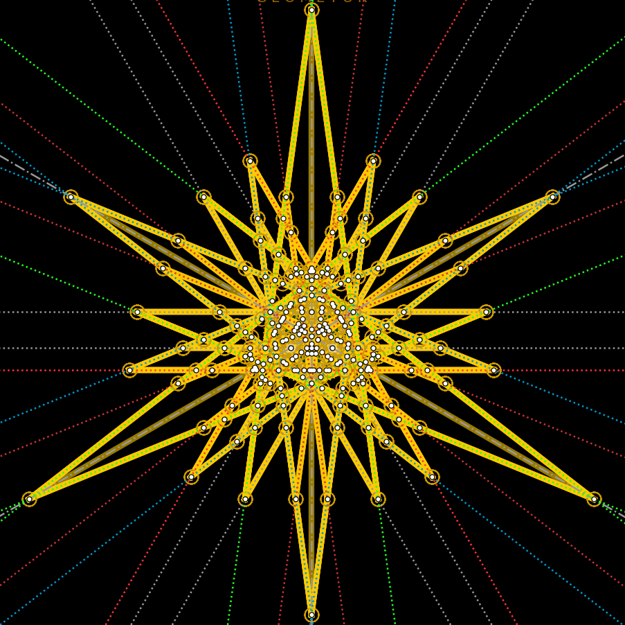
Content of type 'section'

A: (0, \frac{1}{2}) B: (1, \frac{1}{2}) C: (\frac{1}{2}, \frac{1}{2} + \frac{\sqrt{3}}{2}) D: (\frac{1}{2}, \frac{1}{2} - \frac{\sqrt{3}}{2}) E: (\frac{3}{2}, \frac{1}{2} + \frac{\sqrt{3}}{2}) F: (- \frac{1}{2}, \frac{1}{2} + \frac{\sqrt{3}}{2}) G: (\frac{7}{2}, \frac{1}{2}) H: (4, \frac{1}{2} + \frac{\sqrt{3}}{2}) I: (3, \frac{1}{2} + \frac{\sqrt{3}}{2}) J: (\frac{9}{2}, \frac{1}{2}) K: (5, \frac{1}{2} + \frac{\sqrt{3}}{2}) L: (\frac{11}{2}, \frac{1}{2}) M: (4, \frac{1}{2} - \frac{\sqrt{3}}{2}) N: (5, \frac{1}{2} - \frac{\sqrt{3}}{2}) O: (3, \frac{1}{2} - \frac{\sqrt{3}}{2}) P: (\frac{5}{2}, \frac{1}{2}) Q: (8, - \frac{1}{2}) R: (9, - \frac{1}{2}) S: (9, \frac{1}{2}) T: (8, \frac{1}{2}) U: (8, - \frac{3}{2}) V: (9, - \frac{3}{2}) W: (10, - \frac{1}{2}) X: (10, \frac{1}{2}) Y: (9, \frac{3}{2}) Z: (8, \frac{3}{2}) AA: (7, \frac{1}{2}) BB: (7, - \frac{1}{2}) CC: (9, \frac{5}{2}) DD: (8, \frac{5}{2}) Tetrahedron (Fig. 29) Octahedron (Fig. 30) Cube (Fig. 32)

Die Fünf Platonischen & Siben Archimedischen Körpernetze (Fig. 29–43)

Das Viert büchlein. (Camerarius 1532: Liber Quartus — De quinque corporibus regularibus, corporibus irregulariis explicatis, duplicatione cubi ac perspectiva.)

A: (0, \frac{1}{2}) B: (1, \frac{1}{2}) C: (\frac{1}{2}, \frac{1}{2} + \frac{\sqrt{3}}{2}) D: (\frac{1}{2}, \frac{1}{2} - \frac{\sqrt{3}}{2}) E: (\frac{3}{2}, \frac{1}{2} + \frac{\sqrt{3}}{2}) F: (- \frac{1}{2}, \frac{1}{2} + \frac{\sqrt{3}}{2}) G: (\frac{7}{2}, \frac{1}{2}) H: (4, \frac{1}{2} + \frac{\sqrt{3}}{2}) I: (3, \frac{1}{2} + \frac{\sqrt{3}}{2}) J: (\frac{9}{2}, \frac{1}{2}) K: (5, \frac{1}{2} + \frac{\sqrt{3}}{2}) L: (\frac{11}{2}, \frac{1}{2}) M: (4, \frac{1}{2} - \frac{\sqrt{3}}{2}) N: (5, \frac{1}{2} - \frac{\sqrt{3}}{2}) O: (3, \frac{1}{2} - \frac{\sqrt{3}}{2}) P: (\frac{5}{2}, \frac{1}{2}) Q: (8, - \frac{1}{2}) R: (9, - \frac{1}{2}) S: (9, \frac{1}{2}) T: (8, \frac{1}{2}) U: (8, - \frac{3}{2}) V: (9, - \frac{3}{2}) W: (10, - \frac{1}{2}) X: (10, \frac{1}{2}) Y: (9, \frac{3}{2}) Z: (8, \frac{3}{2}) AA: (7, \frac{1}{2}) BB: (7, - \frac{1}{2}) CC: (9, \frac{5}{2}) DD: (8, \frac{5}{2}) Tetrahedron (Fig. 29) Octahedron (Fig. 30) Cube (Fig. 32)

First Printed Planar Fold-Out Nets for Platonic & Archimedean Solids (Figs. 29–43)

In the opening of Book IV, Dürer classifies three families of solid bodies that may be fashioned with compass and straightedge: prismatic columns of uniform cross-section, tapering cones and pyramids, and finally bodies equal on every side in their faces, solid corners, and edges, “which :person:`Euclid <euclid>` calls :term:`corpora regularia <corpora-regularia>`, describing five of them because there can be no more that may be inscribed in a sphere touching it at every vertex” (euclid:elements, plato:timaeus).

A: (0, \frac{1}{2}) B: (1, \frac{1}{2}) C: (\frac{1}{2}, \frac{1}{2} + \frac{\sqrt{3}}{2}) D: (\frac{1}{2}, \frac{1}{2} - \frac{\sqrt{3}}{2}) E: (\frac{3}{2}, \frac{1}{2} + \frac{\sqrt{3}}{2}) F: (- \frac{1}{2}, \frac{1}{2} + \frac{\sqrt{3}}{2}) G: (\frac{7}{2}, \frac{1}{2}) H: (4, \frac{1}{2} + \frac{\sqrt{3}}{2}) I: (3, \frac{1}{2} + \frac{\sqrt{3}}{2}) J: (\frac{9}{2}, \frac{1}{2}) K: (5, \frac{1}{2} + \frac{\sqrt{3}}{2}) L: (\frac{11}{2}, \frac{1}{2}) M: (4, \frac{1}{2} - \frac{\sqrt{3}}{2}) N: (5, \frac{1}{2} - \frac{\sqrt{3}}{2}) O: (3, \frac{1}{2} - \frac{\sqrt{3}}{2}) P: (\frac{5}{2}, \frac{1}{2}) Q: (8, - \frac{1}{2}) R: (9, - \frac{1}{2}) S: (9, \frac{1}{2}) T: (8, \frac{1}{2}) U: (8, - \frac{3}{2}) V: (9, - \frac{3}{2}) W: (10, - \frac{1}{2}) X: (10, \frac{1}{2}) Y: (9, \frac{3}{2}) Z: (8, \frac{3}{2}) AA: (7, \frac{1}{2}) BB: (7, - \frac{1}{2}) CC: (9, \frac{5}{2}) DD: (8, \frac{5}{2}) Tetrahedron (Fig. 29) Octahedron (Fig. 30) Cube (Fig. 32)

Notes — Combinatorics & Topology of Dürer’s Polyhedral Nets

Book IV (pp. 142–157) marks a watershed between Luca Pacioli's Divina Proportione (pacioli:1509)—where Leonardo da Vinci rendered polyhedra as perspective wooden frames—and Johannes Kepler's Harmonices Mundi Book II (kepler:1619), which completed the enumeration of all thirteen Archimedean solids.

Notes — Dedication to Willibald Pirckheimer (1525)

Dürer’s opening dedication to Nuremberg patrician and humanist Willibald Pirckheimer (1470–1530) articulates the core intellectual manifesto of the Northern Renaissance: liberating the German craftsman from unreflective workshop custom (wie eyn wylder vnbeschnytener bawm) through the mathematical rigor of compass and straightedge (die kunst der messung). Written amidst the religious upheavals of 1525, Dürer also mounts a spirited humanist defense of painting against Reformation iconoclasm, insisting that sacred art edifies rather than misleads when governed by rational proportion.

Notes — Plane Enclosure, Corners vs. Angles & Quadrilaterals (Figs. 1–8)

In Book II (Figs. 1–8), Dürer emphasizes the practical craftsman’s operational distinction between looking upon the sharp external vertex (Eck, salient angle) versus looking into the recessed hollow (Winckel, interior cavity). He grounds angle construction in Thales’s semicircle theorem (Fig. 4) and classifies eight species of quadrilaterals (Fierungen)—distinguishing the true square (rechte Fierung) from oblongs, rhombi, rhomboids, and four empirical trapezia.

Notes — Vitruvian Orders, Entasis & Enveloped-Sphere 3D Contours

Book III opens Dürer’s architectural treatise with an homage to Vitruvius (vitruvius:architectura), balanced by the German master’s flair for bold ornamental invention. To define the sinuous three-dimensional contour of a twisted column (Figs. 9–10), Dürer conceives every station along its coiled helical axis as the center of an inscribed sphere (ein yeklicher punct in der gewunden axt der seulen ein centrum einer kugel)—an early practical instance of envelope theory in spatial constructive geometry.

Plane Enclosure, Exterior Corners vs. Interior Angles & Quadrilaterals (Figs. 1–8)

Having shown in the first book how various lines are to be drawn, I now proceed—as promised at the outset—to planes (planos oder ebne felder), and teach how to construct several of their many figures. To understand what a plane figure is: it is a magnitude bounded and set apart by lines that does not yet enclose a solid body (Corpus). Just as lines enclose a plane, so planes enclose solid bodies.

A: (0, \frac{1}{2}) B: (1, \frac{1}{2}) C: (\frac{1}{2}, \frac{1}{2} + \frac{\sqrt{3}}{2}) D: (\frac{1}{2}, \frac{1}{2} - \frac{\sqrt{3}}{2}) E: (\frac{3}{2}, \frac{1}{2} + \frac{\sqrt{3}}{2}) F: (- \frac{1}{2}, \frac{1}{2} + \frac{\sqrt{3}}{2}) G: (\frac{7}{2}, \frac{1}{2}) H: (4, \frac{1}{2} + \frac{\sqrt{3}}{2}) I: (3, \frac{1}{2} + \frac{\sqrt{3}}{2}) J: (\frac{9}{2}, \frac{1}{2}) K: (5, \frac{1}{2} + \frac{\sqrt{3}}{2}) L: (\frac{11}{2}, \frac{1}{2}) M: (4, \frac{1}{2} - \frac{\sqrt{3}}{2}) N: (5, \frac{1}{2} - \frac{\sqrt{3}}{2}) O: (3, \frac{1}{2} - \frac{\sqrt{3}}{2}) P: (\frac{5}{2}, \frac{1}{2}) Q: (8, - \frac{1}{2}) R: (9, - \frac{1}{2}) S: (9, \frac{1}{2}) T: (8, \frac{1}{2}) U: (8, - \frac{3}{2}) V: (9, - \frac{3}{2}) W: (10, - \frac{1}{2}) X: (10, \frac{1}{2}) Y: (9, \frac{3}{2}) Z: (8, \frac{3}{2}) AA: (7, \frac{1}{2}) BB: (7, - \frac{1}{2}) CC: (9, \frac{5}{2}) DD: (8, \frac{5}{2}) Tetrahedron (Fig. 29) Octahedron (Fig. 30) Cube (Fig. 32)

Summary — Planar Nets for Platonic & Archimedean Solids (Figs. 29–43)

First Printed Planar Fold-Out Nets (pp. 142–157, Figs. 29–43):

a: (0, 0) b: (1, 0) d: (\frac{1}{2}, - \frac{\sqrt{3}}{2}) c: (\frac{1}{2}, \frac{\sqrt{3}}{2}) e: (- \frac{1}{2}, - \frac{\sqrt{3}}{2}) f: (\frac{3}{2}, - \frac{\sqrt{3}}{2}) g: (\frac{1}{2}, 1 - \frac{\sqrt{3}}{2}) h: (\frac{1}{4} + \frac{\sqrt{3}}{4} + \frac{\sqrt{2} \sqrt{-2 + 3 \sqrt{3}}}{4}, - \frac{\sqrt{3}}{4} + \frac{\sqrt{2} \sqrt{-2 + 3 \sqrt{3}}}{4} + \frac{3}{4}) i: (- \frac{\sqrt{2} \sqrt{-2 + 3 \sqrt{3}}}{4} - \frac{\sqrt{3}}{4} + \frac{3}{4}, - \frac{\sqrt{3}}{4} + \frac{\sqrt{2} \sqrt{-2 + 3 \sqrt{3}}}{4} + \frac{3}{4}) k: (\frac{- \left(- \frac{\sqrt{2} \sqrt{-2 + 3 \sqrt{3}}}{4} - \frac{\sqrt{3}}{4} + \frac{3}{4}\right)^{2} + \left(- \frac{3}{4} + \frac{\sqrt{3}}{4} + \frac{\sqrt{2} \sqrt{-2 + 3 \sqrt{3}}}{4}\right)^{2} + \left(- \frac{\sqrt{2} \sqrt{-2 + 3 \sqrt{3}}}{2} - \frac{\sqrt{3}}{2} + \frac{1}{2}\right)^{2}}{2 \left(- \frac{\sqrt{2} \sqrt{-2 + 3 \sqrt{3}}}{2} - \frac{\sqrt{3}}{2} + \frac{1}{2}\right)} + \frac{1}{4} + \frac{\sqrt{3}}{4} + \frac{\sqrt{2} \sqrt{-2 + 3 \sqrt{3}}}{4}, - \frac{\sqrt{3}}{4} - \frac{\sqrt{- \left(- \left(- \frac{\sqrt{2} \sqrt{-2 + 3 \sqrt{3}}}{4} - \frac{\sqrt{3}}{4} + \frac{3}{4}\right)^{2} + \left(- \frac{3}{4} + \frac{\sqrt{3}}{4} + \frac{\sqrt{2} \sqrt{-2 + 3 \sqrt{3}}}{4}\right)^{2} + \left(- \frac{\sqrt{2} \sqrt{-2 + 3 \sqrt{3}}}{2} - \frac{\sqrt{3}}{2} + \frac{1}{2}\right)^{2}\right)^{2} + 4 \left(\left(- \frac{3}{4} + \frac{\sqrt{3}}{4} + \frac{\sqrt{2} \sqrt{-2 + 3 \sqrt{3}}}{4}\right)^{2} + \left(- \frac{\sqrt{3}}{4} + \frac{\sqrt{2} \sqrt{-2 + 3 \sqrt{3}}}{4} + \frac{3}{4}\right)^{2}\right) \left(- \frac{\sqrt{2} \sqrt{-2 + 3 \sqrt{3}}}{2} - \frac{\sqrt{3}}{2} + \frac{1}{2}\right)^{2}}}{2 \left(- \frac{\sqrt{2} \sqrt{-2 + 3 \sqrt{3}}}{2} - \frac{\sqrt{3}}{2} + \frac{1}{2}\right)} + \frac{\sqrt{2} \sqrt{-2 + 3 \sqrt{3}}}{4} + \frac{3}{4}) phi: (\frac{1}{2} + \frac{\sqrt{5}}{2}, 0) H_phi: (\frac{\sqrt{5}}{4} + \frac{3}{4}, \frac{\sqrt{2} \sqrt{5 - \sqrt{5}}}{8} + \frac{\sqrt{10} \sqrt{5 - \sqrt{5}}}{8}) I_phi: (\frac{1}{4} - \frac{\sqrt{5}}{4}, \frac{\sqrt{2} \sqrt{5 - \sqrt{5}}}{8} + \frac{\sqrt{10} \sqrt{5 - \sqrt{5}}}{8}) K_phi: (\frac{1}{2}, \frac{\sqrt{2 \sqrt{5} + 5}}{2}) a b d c e f g h i k phi Hphi Iphi Kphi Solid Gold: Dürer Rusty Compass (108.37°) | Dashed Blue: Euclid Q(phi) (108°)

Demonstrative vs. Mechanice Regular Polygons & the Rusty Compass (Figs. 9–20)

Throughout his polygon constructions, Dürer enforces a remarkably modern epistemological boundary between demonstrative constructions proved with exact Euclidean rigor and rapid mechanice workshop approximations (von behendigkeyt wegen in der arbeyt):

a: (0, 0) b: (1, 0) d: (\frac{1}{2}, - \frac{\sqrt{3}}{2}) c: (\frac{1}{2}, \frac{\sqrt{3}}{2}) e: (- \frac{1}{2}, - \frac{\sqrt{3}}{2}) f: (\frac{3}{2}, - \frac{\sqrt{3}}{2}) g: (\frac{1}{2}, 1 - \frac{\sqrt{3}}{2}) h: (\frac{1}{4} + \frac{\sqrt{3}}{4} + \frac{\sqrt{2} \sqrt{-2 + 3 \sqrt{3}}}{4}, - \frac{\sqrt{3}}{4} + \frac{\sqrt{2} \sqrt{-2 + 3 \sqrt{3}}}{4} + \frac{3}{4}) i: (- \frac{\sqrt{2} \sqrt{-2 + 3 \sqrt{3}}}{4} - \frac{\sqrt{3}}{4} + \frac{3}{4}, - \frac{\sqrt{3}}{4} + \frac{\sqrt{2} \sqrt{-2 + 3 \sqrt{3}}}{4} + \frac{3}{4}) k: (\frac{- \left(- \frac{\sqrt{2} \sqrt{-2 + 3 \sqrt{3}}}{4} - \frac{\sqrt{3}}{4} + \frac{3}{4}\right)^{2} + \left(- \frac{3}{4} + \frac{\sqrt{3}}{4} + \frac{\sqrt{2} \sqrt{-2 + 3 \sqrt{3}}}{4}\right)^{2} + \left(- \frac{\sqrt{2} \sqrt{-2 + 3 \sqrt{3}}}{2} - \frac{\sqrt{3}}{2} + \frac{1}{2}\right)^{2}}{2 \left(- \frac{\sqrt{2} \sqrt{-2 + 3 \sqrt{3}}}{2} - \frac{\sqrt{3}}{2} + \frac{1}{2}\right)} + \frac{1}{4} + \frac{\sqrt{3}}{4} + \frac{\sqrt{2} \sqrt{-2 + 3 \sqrt{3}}}{4}, - \frac{\sqrt{3}}{4} - \frac{\sqrt{- \left(- \left(- \frac{\sqrt{2} \sqrt{-2 + 3 \sqrt{3}}}{4} - \frac{\sqrt{3}}{4} + \frac{3}{4}\right)^{2} + \left(- \frac{3}{4} + \frac{\sqrt{3}}{4} + \frac{\sqrt{2} \sqrt{-2 + 3 \sqrt{3}}}{4}\right)^{2} + \left(- \frac{\sqrt{2} \sqrt{-2 + 3 \sqrt{3}}}{2} - \frac{\sqrt{3}}{2} + \frac{1}{2}\right)^{2}\right)^{2} + 4 \left(\left(- \frac{3}{4} + \frac{\sqrt{3}}{4} + \frac{\sqrt{2} \sqrt{-2 + 3 \sqrt{3}}}{4}\right)^{2} + \left(- \frac{\sqrt{3}}{4} + \frac{\sqrt{2} \sqrt{-2 + 3 \sqrt{3}}}{4} + \frac{3}{4}\right)^{2}\right) \left(- \frac{\sqrt{2} \sqrt{-2 + 3 \sqrt{3}}}{2} - \frac{\sqrt{3}}{2} + \frac{1}{2}\right)^{2}}}{2 \left(- \frac{\sqrt{2} \sqrt{-2 + 3 \sqrt{3}}}{2} - \frac{\sqrt{3}}{2} + \frac{1}{2}\right)} + \frac{\sqrt{2} \sqrt{-2 + 3 \sqrt{3}}}{4} + \frac{3}{4}) phi: (\frac{1}{2} + \frac{\sqrt{5}}{2}, 0) H_phi: (\frac{\sqrt{5}}{4} + \frac{3}{4}, \frac{\sqrt{2} \sqrt{5 - \sqrt{5}}}{8} + \frac{\sqrt{10} \sqrt{5 - \sqrt{5}}}{8}) I_phi: (\frac{1}{4} - \frac{\sqrt{5}}{4}, \frac{\sqrt{2} \sqrt{5 - \sqrt{5}}}{8} + \frac{\sqrt{10} \sqrt{5 - \sqrt{5}}}{8}) K_phi: (\frac{1}{2}, \frac{\sqrt{2 \sqrt{5} + 5}}{2}) a b d c e f g h i k phi Hphi Iphi Kphi Solid Gold: Dürer Rusty Compass (108.37°) | Dashed Blue: Euclid Q(phi) (108°)

Notes — Algebraic Audit of Dürer’s Pentagon, Heptagon & 1525 Errata

Why did Dürer present two pentagon constructions back-to-back on pages 058–059 (Figs. 15 and 16)? While Figure 15 gives Ptolemy's exact golden-ratio chord over $\mathbb{Q}(\phi)$, Figure 16 requires never changing the compass opening (auß vnuerruckten zirckel)—a classic medieval stonemasons’ and Islamic workshop protocol going back to Abū al-Wafāʾ (abulwafa:craftsmen) and Matthäus Roriczer (roritzer:1487), which Hermann Staigmüller (staigmuller:1891) and Émile Lemoine (lemoine:1902) celebrated as a milestone of constructive simplicity.

Notes — Point, Elementary Lines & Parallel Curves (Figs. 1–5)

In translating Euclid's Elements Book I definitions (euclid:elements) into German print for the first time, Dürer invents a precise vernacular technical vocabulary: Punct, gerade Lini, Zirckellini, and equidistant Barlinien. Crucially, Dürer augments Euclid’s planar palette with the inflected Schlangenlini (serpentine S-curve) and observes the physical convergence of plumb lines toward the center of the earth—grounding abstract geometry directly in workshop observation.

Notes — Projective Collineation in Gnomonics & Tower Scaling

Both Dürer’s Nuremberg gnomonic projection (Figs. 21–23, mapping uniform $15^\circ$ equatorial hour angles onto tangent lines via $\tan(k \cdot 15^\circ)$ scaled by $\sin 49^\circ$ on the horizontal plane and $\cos 49^\circ$ on a prime-vertical South wall) and his tower-inscription ray pencil (p. 114, mapping uniform visual angles $\theta_k$ onto heights $h_k = D\tan\theta_k$) prepare the reader directly for the central-projection perspective theory of Book IV, and inspired D'Arcy Wentworth Thompson's coordinate transformation grids (thompson:1942).

Nuremberg Sundials (PHOTONMATHPLACEHOLDER000023END Pole) & Optical Tower Scaling (Figs. 20–27)

The Nuremberg Analemma & Truncated-Cube Polyhedral Dial (pp. 108–113, Figs. 20–27): Dividing quadrant b.a.c. into $90^\circ$ ($90 = 3 \times 3 \times 2 \times 5$, Fig. 21), Dürer sets the altitude of the celestial pole at Nuremberg to $49^\circ$ (“also zuᵒ Nüremberg ist sein höch neun vnd vierzig grad”), establishing the right-angled wooden or brass gnomonic triangle a.e.d. containing the polar Axis mundi a.d. ($49^\circ$), the vertical Mauerlini d.e., and the perpendicular Equinoctialis e.f. ($41^\circ$). Projecting a 24-sector equinoctial wheel (Fig. 22) onto tangent lines p.q. and r.s. and transferring radii d.e. and a.e. constructs both the vertical South wall dial (an die aufrecht mauer) and the horizontal dial (auf den orizon, Fig. 23), culminating in an octahedrally chamfered polyhedral cube sundial (Figs. 24–25) whose facets face East, West, South, North, the $49^\circ$ Arctic/Antarctic poles, and the $41^\circ$ equinoctial plane.

a: (0, 0) b: (1, 0) d: (\frac{1}{2}, - \frac{\sqrt{3}}{2}) c: (\frac{1}{2}, \frac{\sqrt{3}}{2}) e: (- \frac{1}{2}, - \frac{\sqrt{3}}{2}) f: (\frac{3}{2}, - \frac{\sqrt{3}}{2}) g: (\frac{1}{2}, 1 - \frac{\sqrt{3}}{2}) h: (\frac{1}{4} + \frac{\sqrt{3}}{4} + \frac{\sqrt{2} \sqrt{-2 + 3 \sqrt{3}}}{4}, - \frac{\sqrt{3}}{4} + \frac{\sqrt{2} \sqrt{-2 + 3 \sqrt{3}}}{4} + \frac{3}{4}) i: (- \frac{\sqrt{2} \sqrt{-2 + 3 \sqrt{3}}}{4} - \frac{\sqrt{3}}{4} + \frac{3}{4}, - \frac{\sqrt{3}}{4} + \frac{\sqrt{2} \sqrt{-2 + 3 \sqrt{3}}}{4} + \frac{3}{4}) k: (\frac{- \left(- \frac{\sqrt{2} \sqrt{-2 + 3 \sqrt{3}}}{4} - \frac{\sqrt{3}}{4} + \frac{3}{4}\right)^{2} + \left(- \frac{3}{4} + \frac{\sqrt{3}}{4} + \frac{\sqrt{2} \sqrt{-2 + 3 \sqrt{3}}}{4}\right)^{2} + \left(- \frac{\sqrt{2} \sqrt{-2 + 3 \sqrt{3}}}{2} - \frac{\sqrt{3}}{2} + \frac{1}{2}\right)^{2}}{2 \left(- \frac{\sqrt{2} \sqrt{-2 + 3 \sqrt{3}}}{2} - \frac{\sqrt{3}}{2} + \frac{1}{2}\right)} + \frac{1}{4} + \frac{\sqrt{3}}{4} + \frac{\sqrt{2} \sqrt{-2 + 3 \sqrt{3}}}{4}, - \frac{\sqrt{3}}{4} - \frac{\sqrt{- \left(- \left(- \frac{\sqrt{2} \sqrt{-2 + 3 \sqrt{3}}}{4} - \frac{\sqrt{3}}{4} + \frac{3}{4}\right)^{2} + \left(- \frac{3}{4} + \frac{\sqrt{3}}{4} + \frac{\sqrt{2} \sqrt{-2 + 3 \sqrt{3}}}{4}\right)^{2} + \left(- \frac{\sqrt{2} \sqrt{-2 + 3 \sqrt{3}}}{2} - \frac{\sqrt{3}}{2} + \frac{1}{2}\right)^{2}\right)^{2} + 4 \left(\left(- \frac{3}{4} + \frac{\sqrt{3}}{4} + \frac{\sqrt{2} \sqrt{-2 + 3 \sqrt{3}}}{4}\right)^{2} + \left(- \frac{\sqrt{3}}{4} + \frac{\sqrt{2} \sqrt{-2 + 3 \sqrt{3}}}{4} + \frac{3}{4}\right)^{2}\right) \left(- \frac{\sqrt{2} \sqrt{-2 + 3 \sqrt{3}}}{2} - \frac{\sqrt{3}}{2} + \frac{1}{2}\right)^{2}}}{2 \left(- \frac{\sqrt{2} \sqrt{-2 + 3 \sqrt{3}}}{2} - \frac{\sqrt{3}}{2} + \frac{1}{2}\right)} + \frac{\sqrt{2} \sqrt{-2 + 3 \sqrt{3}}}{4} + \frac{3}{4}) phi: (\frac{1}{2} + \frac{\sqrt{5}}{2}, 0) H_phi: (\frac{\sqrt{5}}{4} + \frac{3}{4}, \frac{\sqrt{2} \sqrt{5 - \sqrt{5}}}{8} + \frac{\sqrt{10} \sqrt{5 - \sqrt{5}}}{8}) I_phi: (\frac{1}{4} - \frac{\sqrt{5}}{4}, \frac{\sqrt{2} \sqrt{5 - \sqrt{5}}}{8} + \frac{\sqrt{10} \sqrt{5 - \sqrt{5}}}{8}) K_phi: (\frac{1}{2}, \frac{\sqrt{2 \sqrt{5} + 5}}{2}) a b d c e f g h i k phi Hphi Iphi Kphi Solid Gold: Dürer Rusty Compass (108.37°) | Dashed Blue: Euclid Q(phi) (108°)

Sechseck, Sibeneck, Fünffeck (demonstrative & unverruckt), 11- & 13-Eck (Fig. 9–20)

(Camerarius 1532: De figuris aequilateris & aequiangulis — Demonstrative ac Mechanice.)

a: (0, 0) b: (1, 0) d: (\frac{1}{2}, - \frac{\sqrt{3}}{2}) c: (\frac{1}{2}, \frac{\sqrt{3}}{2}) e: (- \frac{1}{2}, - \frac{\sqrt{3}}{2}) f: (\frac{3}{2}, - \frac{\sqrt{3}}{2}) g: (\frac{1}{2}, 1 - \frac{\sqrt{3}}{2}) h: (\frac{1}{4} + \frac{\sqrt{3}}{4} + \frac{\sqrt{2} \sqrt{-2 + 3 \sqrt{3}}}{4}, - \frac{\sqrt{3}}{4} + \frac{\sqrt{2} \sqrt{-2 + 3 \sqrt{3}}}{4} + \frac{3}{4}) i: (- \frac{\sqrt{2} \sqrt{-2 + 3 \sqrt{3}}}{4} - \frac{\sqrt{3}}{4} + \frac{3}{4}, - \frac{\sqrt{3}}{4} + \frac{\sqrt{2} \sqrt{-2 + 3 \sqrt{3}}}{4} + \frac{3}{4}) k: (\frac{- \left(- \frac{\sqrt{2} \sqrt{-2 + 3 \sqrt{3}}}{4} - \frac{\sqrt{3}}{4} + \frac{3}{4}\right)^{2} + \left(- \frac{3}{4} + \frac{\sqrt{3}}{4} + \frac{\sqrt{2} \sqrt{-2 + 3 \sqrt{3}}}{4}\right)^{2} + \left(- \frac{\sqrt{2} \sqrt{-2 + 3 \sqrt{3}}}{2} - \frac{\sqrt{3}}{2} + \frac{1}{2}\right)^{2}}{2 \left(- \frac{\sqrt{2} \sqrt{-2 + 3 \sqrt{3}}}{2} - \frac{\sqrt{3}}{2} + \frac{1}{2}\right)} + \frac{1}{4} + \frac{\sqrt{3}}{4} + \frac{\sqrt{2} \sqrt{-2 + 3 \sqrt{3}}}{4}, - \frac{\sqrt{3}}{4} - \frac{\sqrt{- \left(- \left(- \frac{\sqrt{2} \sqrt{-2 + 3 \sqrt{3}}}{4} - \frac{\sqrt{3}}{4} + \frac{3}{4}\right)^{2} + \left(- \frac{3}{4} + \frac{\sqrt{3}}{4} + \frac{\sqrt{2} \sqrt{-2 + 3 \sqrt{3}}}{4}\right)^{2} + \left(- \frac{\sqrt{2} \sqrt{-2 + 3 \sqrt{3}}}{2} - \frac{\sqrt{3}}{2} + \frac{1}{2}\right)^{2}\right)^{2} + 4 \left(\left(- \frac{3}{4} + \frac{\sqrt{3}}{4} + \frac{\sqrt{2} \sqrt{-2 + 3 \sqrt{3}}}{4}\right)^{2} + \left(- \frac{\sqrt{3}}{4} + \frac{\sqrt{2} \sqrt{-2 + 3 \sqrt{3}}}{4} + \frac{3}{4}\right)^{2}\right) \left(- \frac{\sqrt{2} \sqrt{-2 + 3 \sqrt{3}}}{2} - \frac{\sqrt{3}}{2} + \frac{1}{2}\right)^{2}}}{2 \left(- \frac{\sqrt{2} \sqrt{-2 + 3 \sqrt{3}}}{2} - \frac{\sqrt{3}}{2} + \frac{1}{2}\right)} + \frac{\sqrt{2} \sqrt{-2 + 3 \sqrt{3}}}{4} + \frac{3}{4}) phi: (\frac{1}{2} + \frac{\sqrt{5}}{2}, 0) H_phi: (\frac{\sqrt{5}}{4} + \frac{3}{4}, \frac{\sqrt{2} \sqrt{5 - \sqrt{5}}}{8} + \frac{\sqrt{10} \sqrt{5 - \sqrt{5}}}{8}) I_phi: (\frac{1}{4} - \frac{\sqrt{5}}{4}, \frac{\sqrt{2} \sqrt{5 - \sqrt{5}}}{8} + \frac{\sqrt{10} \sqrt{5 - \sqrt{5}}}{8}) K_phi: (\frac{1}{2}, \frac{\sqrt{2 \sqrt{5} + 5}}{2}) a b d c e f g h i k phi Hphi Iphi Kphi Solid Gold: Dürer Rusty Compass (108.37°) | Dashed Blue: Euclid Q(phi) (108°)

Summary — Demonstrative vs. Mechanice Polygons & Rusty Compass (Figs. 9–20)

Epistemology of Regular Polygons: *Demonstrative* vs. *Mechanice* (pp. 057–061, Figs. 9–20):

The Delian Altar: Doubling the Cube & Cannonball Scaling (Figs. 44–51)

Recounting how the citizens of plague-stricken Athens consulted Apollo’s oracle and were commanded to double his cubical altar, Dürer explains how Plato reduced cube duplication to finding two mean proportionals ($g : c = c : d = d : e \implies c^3 = g^2 e$) between two unequal segments. Declaring that “because this is a most useful art serving all craftsmen, yet kept in great secrecy and concealment by scholars, I wish to bring it into the light of day—for as I believe, it has never until this day been described in the German tongue,” Dürer presents three classical constructions and applies them directly to casting proportional bells and iron cannonballs (püxsen kugeln) of $1, 2, 3, \dots, 100$ pounds:

A': (- \frac{3}{4}, \frac{5}{4}) B': (\frac{9}{4}, \frac{5}{4}) C': (\frac{9}{4}, \frac{17}{4}) D': (- \frac{3}{4}, \frac{17}{4}) E': (0, 2) F': (\frac{12}{5}, 2) G': (\frac{12}{5}, \frac{22}{5}) H': (0, \frac{22}{5}) V_x: (3, 5) M': (- \frac{1}{3}, \frac{5}{3}) A' B' C' D' E' F' G' H' Vx M' Book IV, Figs. 56–63 — Glass Picture Plane Projection (CR(A', E'; M', V_x) = -1)

Cube Sciagraphy & Central Projection Perspective Apparatuses (Figs. 52–63)

Book IV culminates in the geometric synthesis of light, shadow, and central perspective (Perspectiva = Durchsehung):

a: (0, 10) b: (10, 10) c: (0, 0) d: (10, 0) e: (5, 10) f: (5, 0) g: (0, 5) h: (10, 5) i: (1, 0) k: (9, 0) V: (\frac{14}{3}, \frac{200}{21}) S_L: (\frac{3}{2} - \frac{\sqrt{449}}{14}, \frac{10}{7}) S_R: (\frac{\sqrt{449}}{14} + \frac{17}{2}, \frac{10}{7}) a b c d e f g h i k V SL SR Book III, p. 115 — Roman Antiqua A (10x10 Square, 1 : 1/3 Contrast)

Das Lateinisch ABC (Antiqua) & Die Alte Textur (S. 115–141)

(Camerarius 1532: De recta ratione formandarum litterarum Latinarum ac Germanicarum.)

O: (0, 0) P_24: (12, 0) A: (-12, 0) B: (6 \sqrt{3}, 6) C: (- 6 \sqrt{3}, -6) D: (6, 6 \sqrt{3}) E: (-6, - 6 \sqrt{3}) F: (0, 12) G: (0, -12) H: (-6, 6 \sqrt{3}) I: (6, - 6 \sqrt{3}) J: (- 6 \sqrt{3}, 6) K: (6 \sqrt{3}, -6) S1: (\frac{\sqrt{3}}{4}, \frac{1}{4}) S2: (\frac{1}{2}, \frac{\sqrt{3}}{2}) S3: (0, \frac{3}{2}) S4: (-1, \sqrt{3}) S5: (- \frac{5 \sqrt{3}}{4}, \frac{5}{4}) P_6: (-3, 0) S7: (- \frac{7 \sqrt{3}}{4}, - \frac{7}{4}) S8: (-2, - 2 \sqrt{3}) S9: (0, - \frac{9}{2}) S10: (\frac{5}{2}, - \frac{5 \sqrt{3}}{2}) S11: (\frac{11 \sqrt{3}}{4}, - \frac{11}{4}) P_12: (6, 0) S13: (\frac{13 \sqrt{3}}{4}, \frac{13}{4}) S14: (\frac{7}{2}, \frac{7 \sqrt{3}}{2}) S15: (0, \frac{15}{2}) S16: (-4, 4 \sqrt{3}) S17: (- \frac{17 \sqrt{3}}{4}, \frac{17}{4}) P_18: (-9, 0) S19: (- \frac{19 \sqrt{3}}{4}, - \frac{19}{4}) S20: (-5, - 5 \sqrt{3}) S21: (0, - \frac{21}{2}) S22: (\frac{11}{2}, - \frac{11 \sqrt{3}}{2}) S23: (\frac{23 \sqrt{3}}{4}, - \frac{23}{4}) O P24 P6 P12 P18 Book I, Figs. 7 & 17 — 12-Sector Archimedean Schneckenlini

Die Schneckenlini & Ewige Lini (Fig. 7, 17 & 27)

(Camerarius 1532: Linea spiralis sive cochlis.)

a: (0, 10) b: (10, 10) c: (0, 0) d: (10, 0) e: (5, 10) f: (5, 0) g: (0, 5) h: (10, 5) i: (1, 0) k: (9, 0) V: (\frac{14}{3}, \frac{200}{21}) S_L: (\frac{3}{2} - \frac{\sqrt{449}}{14}, \frac{10}{7}) S_R: (\frac{\sqrt{449}}{14} + \frac{17}{2}, \frac{10}{7}) a b c d e f g h i k V SL SR Book III, p. 115 — Roman Antiqua A (10x10 Square, 1 : 1/3 Contrast)

Notes — Constructive Typography: Pacioli vs. Dürer & Textura Pitch

In Divina Proportione (pacioli:1509), Luca Pacioli framed Roman capitals inside a square with a $1 : 9$ stroke-to-height ratio and constructed round letters such as O using four distinct circles (two concentric outer/inner circles or paired ovals). In Book III of the Underweysung (pp. 115–135), Dürer makes three decisive innovations:

Notes — Gothic Tracery, Planar Tilings & Pentagonal Parquetries (Figs. 21–27)

Dürer’s four assemblies of regular pentagons in Book II, Fig. 24 (p. 066)—including antiparallel strips and fivefold rosettes (fünf rosen van den fünf ecken) separated by golden rhombic voids—mark the historical birth of non-periodic fivefold planar parquetries. Dürer explicitly notes on page 068 that edge-joined rings of pentagons or heptagons cannot tile the plane without gaping or overlapping, directly inspiring Johannes Kepler's exploration of semiregular and pentagonal tilings in Book II of Harmonices Mundi (kepler:1619) and anticipating modern Penrose tilings.

A': (- \frac{3}{4}, \frac{5}{4}) B': (\frac{9}{4}, \frac{5}{4}) C': (\frac{9}{4}, \frac{17}{4}) D': (- \frac{3}{4}, \frac{17}{4}) E': (0, 2) F': (\frac{12}{5}, 2) G': (\frac{12}{5}, \frac{22}{5}) H': (0, \frac{22}{5}) V_x: (3, 5) M': (- \frac{1}{3}, \frac{5}{3}) A' B' C' D' E' F' G' H' Vx M' Book IV, Figs. 56–63 — Glass Picture Plane Projection (CR(A', E'; M', V_x) = -1)

Notes — Homogeneous Central Projection & Cross-Ratio Invariance

In construct_durer_perspective_apparatus(), let the artist’s fixed eye point be $E = (-12, 3, 5)$ looking orthogonally toward the vertical glass picture frame $x = 0$ (principal vanishing point $V_x = (3, 5)$ on the glass, focal distance $f = 12$). Every vertex $P = (X, Y, Z) \in \mathbb{Q}^3$ projects along rectilinear sight-ray $EP$ to exact rational picture-plane coordinates:

O: (0, 0) P_24: (12, 0) A: (-12, 0) B: (6 \sqrt{3}, 6) C: (- 6 \sqrt{3}, -6) D: (6, 6 \sqrt{3}) E: (-6, - 6 \sqrt{3}) F: (0, 12) G: (0, -12) H: (-6, 6 \sqrt{3}) I: (6, - 6 \sqrt{3}) J: (- 6 \sqrt{3}, 6) K: (6 \sqrt{3}, -6) S1: (\frac{\sqrt{3}}{4}, \frac{1}{4}) S2: (\frac{1}{2}, \frac{\sqrt{3}}{2}) S3: (0, \frac{3}{2}) S4: (-1, \sqrt{3}) S5: (- \frac{5 \sqrt{3}}{4}, \frac{5}{4}) P_6: (-3, 0) S7: (- \frac{7 \sqrt{3}}{4}, - \frac{7}{4}) S8: (-2, - 2 \sqrt{3}) S9: (0, - \frac{9}{2}) S10: (\frac{5}{2}, - \frac{5 \sqrt{3}}{2}) S11: (\frac{11 \sqrt{3}}{4}, - \frac{11}{4}) P_12: (6, 0) S13: (\frac{13 \sqrt{3}}{4}, \frac{13}{4}) S14: (\frac{7}{2}, \frac{7 \sqrt{3}}{2}) S15: (0, \frac{15}{2}) S16: (-4, 4 \sqrt{3}) S17: (- \frac{17 \sqrt{3}}{4}, \frac{17}{4}) P_18: (-9, 0) S19: (- \frac{19 \sqrt{3}}{4}, - \frac{19}{4}) S20: (-5, - 5 \sqrt{3}) S21: (0, - \frac{21}{2}) S22: (\frac{11}{2}, - \frac{11 \sqrt{3}}{2}) S23: (\frac{23 \sqrt{3}}{4}, - \frac{23}{4}) O P24 P6 P12 P18 Book I, Figs. 7 & 17 — 12-Sector Archimedean Schneckenlini

Notes — Planar Spirals, Volutes & Spatial Helices (Figs. 6–27)

Because $\cos(k \cdot 30^\circ), \sin(k \cdot 30^\circ) \in \left\{0, \pm\frac{1}{2}, \pm\frac{\sqrt{3}}{2}, \pm 1\right\}$ for every integer $k$, all 25 stations of Dürer’s two-turn 12-sector Archimedean spiral $P_k = \left(\frac{k}{2}\cos\frac{k\pi}{6},\, \frac{k}{2}\sin\frac{k\pi}{6}\right)$ belong entirely to the quadratic field $\mathbb{Q}(\sqrt{3})$, requiring zero floating-point evaluation in geometor.model.

O: (0, 0) P_24: (12, 0) A: (-12, 0) B: (6 \sqrt{3}, 6) C: (- 6 \sqrt{3}, -6) D: (6, 6 \sqrt{3}) E: (-6, - 6 \sqrt{3}) F: (0, 12) G: (0, -12) H: (-6, 6 \sqrt{3}) I: (6, - 6 \sqrt{3}) J: (- 6 \sqrt{3}, 6) K: (6 \sqrt{3}, -6) S1: (\frac{\sqrt{3}}{4}, \frac{1}{4}) S2: (\frac{1}{2}, \frac{\sqrt{3}}{2}) S3: (0, \frac{3}{2}) S4: (-1, \sqrt{3}) S5: (- \frac{5 \sqrt{3}}{4}, \frac{5}{4}) P_6: (-3, 0) S7: (- \frac{7 \sqrt{3}}{4}, - \frac{7}{4}) S8: (-2, - 2 \sqrt{3}) S9: (0, - \frac{9}{2}) S10: (\frac{5}{2}, - \frac{5 \sqrt{3}}{2}) S11: (\frac{11 \sqrt{3}}{4}, - \frac{11}{4}) P_12: (6, 0) S13: (\frac{13 \sqrt{3}}{4}, \frac{13}{4}) S14: (\frac{7}{2}, \frac{7 \sqrt{3}}{2}) S15: (0, \frac{15}{2}) S16: (-4, 4 \sqrt{3}) S17: (- \frac{17 \sqrt{3}}{4}, \frac{17}{4}) P_18: (-9, 0) S19: (- \frac{19 \sqrt{3}}{4}, - \frac{19}{4}) S20: (-5, - 5 \sqrt{3}) S21: (0, - \frac{21}{2}) S22: (\frac{11}{2}, - \frac{11 \sqrt{3}}{2}) S23: (\frac{23 \sqrt{3}}{4}, - \frac{23}{4}) O P24 P6 P12 P18 Book I, Figs. 7 & 17 — 12-Sector Archimedean Schneckenlini

Planar Spirals (Schneckenlinien), Volutes & Spatial Helices (Figs. 6–27)

To draw a true snail-shell spiral (Schneckenlini, archimedes:spirals) beginning at center O (Dürer’s .a.) and expanding uniformly outward (Figs. 7 & 17):

a: (0, 10) b: (10, 10) c: (0, 0) d: (10, 0) e: (5, 10) f: (5, 0) g: (0, 5) h: (10, 5) i: (1, 0) k: (9, 0) V: (\frac{14}{3}, \frac{200}{21}) S_L: (\frac{3}{2} - \frac{\sqrt{449}}{14}, \frac{10}{7}) S_R: (\frac{\sqrt{449}}{14} + \frac{17}{2}, \frac{10}{7}) a b c d e f g h i k V SL SR Book III, p. 115 — Roman Antiqua A (10x10 Square, 1 : 1/3 Contrast)

Roman Antiqua Capitals (A–Z) & Modular Gothic Textura

Because builders and painters inscribe letters on high walls and monuments, Dürer devotes pages 115–141 to the first printed northern Renaissance geometric construction of both Roman capitals (*ein Lateinisch abc*) and Gothic blackletter (*Textur*).

A': (- \frac{3}{4}, \frac{5}{4}) B': (\frac{9}{4}, \frac{5}{4}) C': (\frac{9}{4}, \frac{17}{4}) D': (- \frac{3}{4}, \frac{17}{4}) E': (0, 2) F': (\frac{12}{5}, 2) G': (\frac{12}{5}, \frac{22}{5}) H': (0, \frac{22}{5}) V_x: (3, 5) M': (- \frac{1}{3}, \frac{5}{3}) A' B' C' D' E' F' G' H' Vx M' Book IV, Figs. 56–63 — Glass Picture Plane Projection (CR(A', E'; M', V_x) = -1)

Schattenwurf, Durchsichtige Abschneydung & Glasrahmen-Instrument (Fig. 52–63)

(Camerarius 1532: Sciagraphia cubi, Perspectivae ratio ac Machinae opticae.)

A': (- \frac{3}{4}, \frac{5}{4}) B': (\frac{9}{4}, \frac{5}{4}) C': (\frac{9}{4}, \frac{17}{4}) D': (- \frac{3}{4}, \frac{17}{4}) E': (0, 2) F': (\frac{12}{5}, 2) G': (\frac{12}{5}, \frac{22}{5}) H': (0, \frac{22}{5}) V_x: (3, 5) M': (- \frac{1}{3}, \frac{5}{3}) A' B' C' D' E' F' G' H' Vx M' Book IV, Figs. 56–63 — Glass Picture Plane Projection (CR(A', E'; M', V_x) = -1)

Summary — Cube Sciagraphy & Perspective Apparatuses (Figs. 52–63)

Cube Sciagraphy, Central Perspective & Optical Machines (pp. 166–182, Figs. 52–63):

O: (0, 0) P_24: (12, 0) A: (-12, 0) B: (6 \sqrt{3}, 6) C: (- 6 \sqrt{3}, -6) D: (6, 6 \sqrt{3}) E: (-6, - 6 \sqrt{3}) F: (0, 12) G: (0, -12) H: (-6, 6 \sqrt{3}) I: (6, - 6 \sqrt{3}) J: (- 6 \sqrt{3}, 6) K: (6 \sqrt{3}, -6) S1: (\frac{\sqrt{3}}{4}, \frac{1}{4}) S2: (\frac{1}{2}, \frac{\sqrt{3}}{2}) S3: (0, \frac{3}{2}) S4: (-1, \sqrt{3}) S5: (- \frac{5 \sqrt{3}}{4}, \frac{5}{4}) P_6: (-3, 0) S7: (- \frac{7 \sqrt{3}}{4}, - \frac{7}{4}) S8: (-2, - 2 \sqrt{3}) S9: (0, - \frac{9}{2}) S10: (\frac{5}{2}, - \frac{5 \sqrt{3}}{2}) S11: (\frac{11 \sqrt{3}}{4}, - \frac{11}{4}) P_12: (6, 0) S13: (\frac{13 \sqrt{3}}{4}, \frac{13}{4}) S14: (\frac{7}{2}, \frac{7 \sqrt{3}}{2}) S15: (0, \frac{15}{2}) S16: (-4, 4 \sqrt{3}) S17: (- \frac{17 \sqrt{3}}{4}, \frac{17}{4}) P_18: (-9, 0) S19: (- \frac{19 \sqrt{3}}{4}, - \frac{19}{4}) S20: (-5, - 5 \sqrt{3}) S21: (0, - \frac{21}{2}) S22: (\frac{11}{2}, - \frac{11 \sqrt{3}}{2}) S23: (\frac{23 \sqrt{3}}{4}, - \frac{23}{4}) O P24 P6 P12 P18 Book I, Figs. 7 & 17 — 12-Sector Archimedean Schneckenlini

Summary — Planar Spirals, Volutes & Spatial Helices (Figs. 6–27)

Planar Spirals, Projective Volutes & Spatial Helices (pp. 010–029, Figs. 6–27):

a: (0, 10) b: (10, 10) c: (0, 0) d: (10, 0) e: (5, 10) f: (5, 0) g: (0, 5) h: (10, 5) i: (1, 0) k: (9, 0) V: (\frac{14}{3}, \frac{200}{21}) S_L: (\frac{3}{2} - \frac{\sqrt{449}}{14}, \frac{10}{7}) S_R: (\frac{\sqrt{449}}{14} + \frac{17}{2}, \frac{10}{7}) a b c d e f g h i k V SL SR Book III, p. 115 — Roman Antiqua A (10x10 Square, 1 : 1/3 Contrast)

Summary — Roman Antiqua Capitals & Modular Gothic Textura

Constructive Typography: Roman *Antiqua* & Modular *Textura* (pp. 115–141):

a: (0, 12) b: (-6, 0) c: (6, 0) f: (-4, 4) g: (2, 8) O_plan: (0, -9) A: (6, -9) B: (4, 4) C: (12, 0) D: (- \frac{7}{2}, \frac{13}{3}) E: (- \frac{23}{6}, \frac{13}{3}) F: (\frac{23}{6}, \frac{13}{3}) G: (\frac{\sqrt{22}}{3} + 12, \frac{\sqrt{13}}{6}) H: (12 - \frac{\sqrt{22}}{3}, \frac{\sqrt{13}}{6}) I: (-3, \frac{14}{3}) J: (- \frac{11}{3}, \frac{14}{3}) K: (\frac{11}{3}, \frac{14}{3}) L: (-3, -9 + \frac{2 \sqrt{10}}{3}) M: (-3, -9 - \frac{2 \sqrt{10}}{3}) N: (\frac{11}{3}, -9) O: (\frac{2 \sqrt{10}}{3} + 12, \frac{\sqrt{13}}{3}) P: (12 - \frac{2 \sqrt{10}}{3}, \frac{\sqrt{13}}{3}) Q: (- \frac{5}{2}, 5) R: (- \frac{7}{2}, 5) S: (\frac{7}{2}, 5) T: (\sqrt{6} + 12, \frac{\sqrt{13}}{2}) U: (12 - \sqrt{6}, \frac{\sqrt{13}}{2}) V: (-2, \frac{16}{3}) W: (- \frac{10}{3}, \frac{16}{3}) X: (\frac{10}{3}, \frac{16}{3}) Y: (-2, - \frac{19}{3}) Z: (-2, - \frac{35}{3}) AA: (\frac{10}{3}, -9) BB: (\frac{44}{3}, \frac{2 \sqrt{13}}{3}) CC: (\frac{28}{3}, \frac{2 \sqrt{13}}{3}) DD: (- \frac{3}{2}, \frac{17}{3}) EE: (- \frac{19}{6}, \frac{17}{3}) FF: (\frac{19}{6}, \frac{17}{3}) GG: (\frac{\sqrt{70}}{3} + 12, \frac{5 \sqrt{13}}{6}) HH: (12 - \frac{\sqrt{70}}{3}, \frac{5 \sqrt{13}}{6}) II: (-1, 6) JJ: (-3, 6) KK: (3, 6) LL: (-1, -9 + 2 \sqrt{2}) MM: (-1, -9 - 2 \sqrt{2}) NN: (3, -9) OO: (2 \sqrt{2} + 12, \sqrt{13}) PP: (12 - 2 \sqrt{2}, \sqrt{13}) QQ: (- \frac{1}{2}, \frac{19}{3}) RR: (- \frac{17}{6}, \frac{19}{3}) SS: (\frac{17}{6}, \frac{19}{3}) TT: (\frac{\sqrt{70}}{3} + 12, \frac{7 \sqrt{13}}{6}) UU: (12 - \frac{\sqrt{70}}{3}, \frac{7 \sqrt{13}}{6}) VV: (0, \frac{20}{3}) WW: (- \frac{8}{3}, \frac{20}{3}) XX: (\frac{8}{3}, \frac{20}{3}) YY: (0, - \frac{19}{3}) ZZ: (0, - \frac{35}{3}) AAA: (\frac{8}{3}, -9) BBB: (\frac{44}{3}, \frac{4 \sqrt{13}}{3}) CCC: (\frac{28}{3}, \frac{4 \sqrt{13}}{3}) DDD: (\frac{1}{2}, 7) EEE: (- \frac{5}{2}, 7) FFF: (\frac{5}{2}, 7) GGG: (\sqrt{6} + 12, \frac{3 \sqrt{13}}{2}) HHH: (12 - \sqrt{6}, \frac{3 \sqrt{13}}{2}) III: (1, \frac{22}{3}) JJJ: (- \frac{7}{3}, \frac{22}{3}) KKK: (\frac{7}{3}, \frac{22}{3}) LLL: (1, -9 + \frac{2 \sqrt{10}}{3}) MMM: (1, -9 - \frac{2 \sqrt{10}}{3}) NNN: (\frac{7}{3}, -9) OOO: (\frac{2 \sqrt{10}}{3} + 12, \frac{5 \sqrt{13}}{3}) PPP: (12 - \frac{2 \sqrt{10}}{3}, \frac{5 \sqrt{13}}{3}) QQQ: (\frac{3}{2}, \frac{23}{3}) RRR: (- \frac{13}{6}, \frac{23}{3}) SSS: (\frac{13}{6}, \frac{23}{3}) TTT: (\frac{\sqrt{22}}{3} + 12, \frac{11 \sqrt{13}}{6}) UUU: (12 - \frac{\sqrt{22}}{3}, \frac{11 \sqrt{13}}{6}) VVV: (-2, 8) WWW: (12, 2 \sqrt{13}) a b c f g Oplan Aufriss (Elevation Cone) Grundriss (Circular Plan) Elipsis / Eierlini (w_k = w_{12-k})

Die drey Kegelschnitte: Elipsis, Parabola, Hiperbole & Muschellini (Fig. 34–40)

(Camerarius 1532: Sectiones coni — Ellipsis, Parabola, Hyperbola; Linea conchois.)

a: (0, 0) b: (1, 0) c: (-1, 0) d: (\frac{1}{2}, \frac{\sqrt{3}}{2}) e: (\frac{1}{2}, 0) W_0: (0, 1) W_1: (- \frac{\sqrt{39}}{8}, \frac{5}{8}) W_2: (- \frac{5 \sqrt{39}}{32}, - \frac{7}{32}) W_6: (\frac{1035 \sqrt{39}}{8192}, \frac{5033}{8192}) O_q: (\frac{14}{5}, 0) a b c d e W0 W1 W2 W6 Oq Heptagon: s_7 = sqrt(3)/2 R (P_7(3/4) = -1/64) Quadrature: d = (8/10) diag => pi = 25/8 = 3.125

Euclidean Area Transformations & Circle Quadrature (Figs. 28–36)

The closing movement of Book II treats comparison and transformation of plane areas (vergleichung der ebnen):

a: (0, 0) b: (1, 0) c: (-1, 0) d: (\frac{1}{2}, \frac{\sqrt{3}}{2}) e: (\frac{1}{2}, 0) W_0: (0, 1) W_1: (- \frac{\sqrt{39}}{8}, \frac{5}{8}) W_2: (- \frac{5 \sqrt{39}}{32}, - \frac{7}{32}) W_6: (\frac{1035 \sqrt{39}}{8192}, \frac{5033}{8192}) O_q: (\frac{14}{5}, 0) a b c d e W0 W1 W2 W6 Oq Heptagon: s_7 = sqrt(3)/2 R (P_7(3/4) = -1/64) Quadrature: d = (8/10) diag => pi = 25/8 = 3.125

Notes — Circle Quadrature & PHOTONMATHPLACEHOLDER000006END (Fig. 34)

For a square of side $a$ and area $a^2$, the diagonal (ortstrich) has length $a\sqrt{2}$. Taking $d = \frac{8}{10}\,a\sqrt{2} = \frac{4\sqrt{2}}{5}a$ gives radius $r = frac{2sqrt{2}}{5}a = sqrt{frac{8}{25}},a$. Equating $\pi_{\text{Dürer}}\,r^2 = a^2$ yields

a: (0, 12) b: (-6, 0) c: (6, 0) f: (-4, 4) g: (2, 8) O_plan: (0, -9) A: (6, -9) B: (4, 4) C: (12, 0) D: (- \frac{7}{2}, \frac{13}{3}) E: (- \frac{23}{6}, \frac{13}{3}) F: (\frac{23}{6}, \frac{13}{3}) G: (\frac{\sqrt{22}}{3} + 12, \frac{\sqrt{13}}{6}) H: (12 - \frac{\sqrt{22}}{3}, \frac{\sqrt{13}}{6}) I: (-3, \frac{14}{3}) J: (- \frac{11}{3}, \frac{14}{3}) K: (\frac{11}{3}, \frac{14}{3}) L: (-3, -9 + \frac{2 \sqrt{10}}{3}) M: (-3, -9 - \frac{2 \sqrt{10}}{3}) N: (\frac{11}{3}, -9) O: (\frac{2 \sqrt{10}}{3} + 12, \frac{\sqrt{13}}{3}) P: (12 - \frac{2 \sqrt{10}}{3}, \frac{\sqrt{13}}{3}) Q: (- \frac{5}{2}, 5) R: (- \frac{7}{2}, 5) S: (\frac{7}{2}, 5) T: (\sqrt{6} + 12, \frac{\sqrt{13}}{2}) U: (12 - \sqrt{6}, \frac{\sqrt{13}}{2}) V: (-2, \frac{16}{3}) W: (- \frac{10}{3}, \frac{16}{3}) X: (\frac{10}{3}, \frac{16}{3}) Y: (-2, - \frac{19}{3}) Z: (-2, - \frac{35}{3}) AA: (\frac{10}{3}, -9) BB: (\frac{44}{3}, \frac{2 \sqrt{13}}{3}) CC: (\frac{28}{3}, \frac{2 \sqrt{13}}{3}) DD: (- \frac{3}{2}, \frac{17}{3}) EE: (- \frac{19}{6}, \frac{17}{3}) FF: (\frac{19}{6}, \frac{17}{3}) GG: (\frac{\sqrt{70}}{3} + 12, \frac{5 \sqrt{13}}{6}) HH: (12 - \frac{\sqrt{70}}{3}, \frac{5 \sqrt{13}}{6}) II: (-1, 6) JJ: (-3, 6) KK: (3, 6) LL: (-1, -9 + 2 \sqrt{2}) MM: (-1, -9 - 2 \sqrt{2}) NN: (3, -9) OO: (2 \sqrt{2} + 12, \sqrt{13}) PP: (12 - 2 \sqrt{2}, \sqrt{13}) QQ: (- \frac{1}{2}, \frac{19}{3}) RR: (- \frac{17}{6}, \frac{19}{3}) SS: (\frac{17}{6}, \frac{19}{3}) TT: (\frac{\sqrt{70}}{3} + 12, \frac{7 \sqrt{13}}{6}) UU: (12 - \frac{\sqrt{70}}{3}, \frac{7 \sqrt{13}}{6}) VV: (0, \frac{20}{3}) WW: (- \frac{8}{3}, \frac{20}{3}) XX: (\frac{8}{3}, \frac{20}{3}) YY: (0, - \frac{19}{3}) ZZ: (0, - \frac{35}{3}) AAA: (\frac{8}{3}, -9) BBB: (\frac{44}{3}, \frac{4 \sqrt{13}}{3}) CCC: (\frac{28}{3}, \frac{4 \sqrt{13}}{3}) DDD: (\frac{1}{2}, 7) EEE: (- \frac{5}{2}, 7) FFF: (\frac{5}{2}, 7) GGG: (\sqrt{6} + 12, \frac{3 \sqrt{13}}{2}) HHH: (12 - \sqrt{6}, \frac{3 \sqrt{13}}{2}) III: (1, \frac{22}{3}) JJJ: (- \frac{7}{3}, \frac{22}{3}) KKK: (\frac{7}{3}, \frac{22}{3}) LLL: (1, -9 + \frac{2 \sqrt{10}}{3}) MMM: (1, -9 - \frac{2 \sqrt{10}}{3}) NNN: (\frac{7}{3}, -9) OOO: (\frac{2 \sqrt{10}}{3} + 12, \frac{5 \sqrt{13}}{3}) PPP: (12 - \frac{2 \sqrt{10}}{3}, \frac{5 \sqrt{13}}{3}) QQQ: (\frac{3}{2}, \frac{23}{3}) RRR: (- \frac{13}{6}, \frac{23}{3}) SSS: (\frac{13}{6}, \frac{23}{3}) TTT: (\frac{\sqrt{22}}{3} + 12, \frac{11 \sqrt{13}}{6}) UUU: (12 - \frac{\sqrt{22}}{3}, \frac{11 \sqrt{13}}{6}) VVV: (-2, 8) WWW: (12, 2 \sqrt{13}) a b c f g Oplan Aufriss (Elevation Cone) Grundriss (Circular Plan) Elipsis / Eierlini (w_k = w_{12-k})

Notes — Two-View Conic Sections & the Eierlini Symmetry Proof

Before Gaspard Monge's Géométrie descriptive (monge:1799), stonecutters and architects knew empirical plan-and-elevation templates, and Piero della Francesca applied coupled projections to human heads in De prospectiva pingendi. Yet Book I, Figures 34–37 of Dürer’s 1525 Underweysung represent the first printed mathematical application of coupled orthographic elevation and ground-plan views to determine the true metric locus of curved three-dimensional sections.

a: (0, 0) b: (1, 0) c: (-1, 0) d: (\frac{1}{2}, \frac{\sqrt{3}}{2}) e: (\frac{1}{2}, 0) W_0: (0, 1) W_1: (- \frac{\sqrt{39}}{8}, \frac{5}{8}) W_2: (- \frac{5 \sqrt{39}}{32}, - \frac{7}{32}) W_6: (\frac{1035 \sqrt{39}}{8192}, \frac{5033}{8192}) O_q: (\frac{14}{5}, 0) a b c d e W0 W1 W2 W6 Oq Heptagon: s_7 = sqrt(3)/2 R (P_7(3/4) = -1/64) Quadrature: d = (8/10) diag => pi = 25/8 = 3.125

Summary — Euclidean Area Transformations & Circle Quadrature (Figs. 28–36)

Area Transformations & Circle Quadrature (pp. 071–076, Figs. 28–36):

a: (0, 12) b: (-6, 0) c: (6, 0) f: (-4, 4) g: (2, 8) O_plan: (0, -9) A: (6, -9) B: (4, 4) C: (12, 0) D: (- \frac{7}{2}, \frac{13}{3}) E: (- \frac{23}{6}, \frac{13}{3}) F: (\frac{23}{6}, \frac{13}{3}) G: (\frac{\sqrt{22}}{3} + 12, \frac{\sqrt{13}}{6}) H: (12 - \frac{\sqrt{22}}{3}, \frac{\sqrt{13}}{6}) I: (-3, \frac{14}{3}) J: (- \frac{11}{3}, \frac{14}{3}) K: (\frac{11}{3}, \frac{14}{3}) L: (-3, -9 + \frac{2 \sqrt{10}}{3}) M: (-3, -9 - \frac{2 \sqrt{10}}{3}) N: (\frac{11}{3}, -9) O: (\frac{2 \sqrt{10}}{3} + 12, \frac{\sqrt{13}}{3}) P: (12 - \frac{2 \sqrt{10}}{3}, \frac{\sqrt{13}}{3}) Q: (- \frac{5}{2}, 5) R: (- \frac{7}{2}, 5) S: (\frac{7}{2}, 5) T: (\sqrt{6} + 12, \frac{\sqrt{13}}{2}) U: (12 - \sqrt{6}, \frac{\sqrt{13}}{2}) V: (-2, \frac{16}{3}) W: (- \frac{10}{3}, \frac{16}{3}) X: (\frac{10}{3}, \frac{16}{3}) Y: (-2, - \frac{19}{3}) Z: (-2, - \frac{35}{3}) AA: (\frac{10}{3}, -9) BB: (\frac{44}{3}, \frac{2 \sqrt{13}}{3}) CC: (\frac{28}{3}, \frac{2 \sqrt{13}}{3}) DD: (- \frac{3}{2}, \frac{17}{3}) EE: (- \frac{19}{6}, \frac{17}{3}) FF: (\frac{19}{6}, \frac{17}{3}) GG: (\frac{\sqrt{70}}{3} + 12, \frac{5 \sqrt{13}}{6}) HH: (12 - \frac{\sqrt{70}}{3}, \frac{5 \sqrt{13}}{6}) II: (-1, 6) JJ: (-3, 6) KK: (3, 6) LL: (-1, -9 + 2 \sqrt{2}) MM: (-1, -9 - 2 \sqrt{2}) NN: (3, -9) OO: (2 \sqrt{2} + 12, \sqrt{13}) PP: (12 - 2 \sqrt{2}, \sqrt{13}) QQ: (- \frac{1}{2}, \frac{19}{3}) RR: (- \frac{17}{6}, \frac{19}{3}) SS: (\frac{17}{6}, \frac{19}{3}) TT: (\frac{\sqrt{70}}{3} + 12, \frac{7 \sqrt{13}}{6}) UU: (12 - \frac{\sqrt{70}}{3}, \frac{7 \sqrt{13}}{6}) VV: (0, \frac{20}{3}) WW: (- \frac{8}{3}, \frac{20}{3}) XX: (\frac{8}{3}, \frac{20}{3}) YY: (0, - \frac{19}{3}) ZZ: (0, - \frac{35}{3}) AAA: (\frac{8}{3}, -9) BBB: (\frac{44}{3}, \frac{4 \sqrt{13}}{3}) CCC: (\frac{28}{3}, \frac{4 \sqrt{13}}{3}) DDD: (\frac{1}{2}, 7) EEE: (- \frac{5}{2}, 7) FFF: (\frac{5}{2}, 7) GGG: (\sqrt{6} + 12, \frac{3 \sqrt{13}}{2}) HHH: (12 - \sqrt{6}, \frac{3 \sqrt{13}}{2}) III: (1, \frac{22}{3}) JJJ: (- \frac{7}{3}, \frac{22}{3}) KKK: (\frac{7}{3}, \frac{22}{3}) LLL: (1, -9 + \frac{2 \sqrt{10}}{3}) MMM: (1, -9 - \frac{2 \sqrt{10}}{3}) NNN: (\frac{7}{3}, -9) OOO: (\frac{2 \sqrt{10}}{3} + 12, \frac{5 \sqrt{13}}{3}) PPP: (12 - \frac{2 \sqrt{10}}{3}, \frac{5 \sqrt{13}}{3}) QQQ: (\frac{3}{2}, \frac{23}{3}) RRR: (- \frac{13}{6}, \frac{23}{3}) SSS: (\frac{13}{6}, \frac{23}{3}) TTT: (\frac{\sqrt{22}}{3} + 12, \frac{11 \sqrt{13}}{6}) UUU: (12 - \frac{\sqrt{22}}{3}, \frac{11 \sqrt{13}}{6}) VVV: (-2, 8) WWW: (12, 2 \sqrt{13}) a b c f g Oplan Aufriss (Elevation Cone) Grundriss (Circular Plan) Elipsis / Eierlini (w_k = w_{12-k})

Summary — Two-View Conic Sections & Kinematic Curves (Figs. 34–42)

Invention of Two-View Descriptive Geometry for Conic Sections (pp. 034–039, Figs. 34–37):

a: (0, 12) b: (-6, 0) c: (6, 0) f: (-4, 4) g: (2, 8) O_plan: (0, -9) A: (6, -9) B: (4, 4) C: (12, 0) D: (- \frac{7}{2}, \frac{13}{3}) E: (- \frac{23}{6}, \frac{13}{3}) F: (\frac{23}{6}, \frac{13}{3}) G: (\frac{\sqrt{22}}{3} + 12, \frac{\sqrt{13}}{6}) H: (12 - \frac{\sqrt{22}}{3}, \frac{\sqrt{13}}{6}) I: (-3, \frac{14}{3}) J: (- \frac{11}{3}, \frac{14}{3}) K: (\frac{11}{3}, \frac{14}{3}) L: (-3, -9 + \frac{2 \sqrt{10}}{3}) M: (-3, -9 - \frac{2 \sqrt{10}}{3}) N: (\frac{11}{3}, -9) O: (\frac{2 \sqrt{10}}{3} + 12, \frac{\sqrt{13}}{3}) P: (12 - \frac{2 \sqrt{10}}{3}, \frac{\sqrt{13}}{3}) Q: (- \frac{5}{2}, 5) R: (- \frac{7}{2}, 5) S: (\frac{7}{2}, 5) T: (\sqrt{6} + 12, \frac{\sqrt{13}}{2}) U: (12 - \sqrt{6}, \frac{\sqrt{13}}{2}) V: (-2, \frac{16}{3}) W: (- \frac{10}{3}, \frac{16}{3}) X: (\frac{10}{3}, \frac{16}{3}) Y: (-2, - \frac{19}{3}) Z: (-2, - \frac{35}{3}) AA: (\frac{10}{3}, -9) BB: (\frac{44}{3}, \frac{2 \sqrt{13}}{3}) CC: (\frac{28}{3}, \frac{2 \sqrt{13}}{3}) DD: (- \frac{3}{2}, \frac{17}{3}) EE: (- \frac{19}{6}, \frac{17}{3}) FF: (\frac{19}{6}, \frac{17}{3}) GG: (\frac{\sqrt{70}}{3} + 12, \frac{5 \sqrt{13}}{6}) HH: (12 - \frac{\sqrt{70}}{3}, \frac{5 \sqrt{13}}{6}) II: (-1, 6) JJ: (-3, 6) KK: (3, 6) LL: (-1, -9 + 2 \sqrt{2}) MM: (-1, -9 - 2 \sqrt{2}) NN: (3, -9) OO: (2 \sqrt{2} + 12, \sqrt{13}) PP: (12 - 2 \sqrt{2}, \sqrt{13}) QQ: (- \frac{1}{2}, \frac{19}{3}) RR: (- \frac{17}{6}, \frac{19}{3}) SS: (\frac{17}{6}, \frac{19}{3}) TT: (\frac{\sqrt{70}}{3} + 12, \frac{7 \sqrt{13}}{6}) UU: (12 - \frac{\sqrt{70}}{3}, \frac{7 \sqrt{13}}{6}) VV: (0, \frac{20}{3}) WW: (- \frac{8}{3}, \frac{20}{3}) XX: (\frac{8}{3}, \frac{20}{3}) YY: (0, - \frac{19}{3}) ZZ: (0, - \frac{35}{3}) AAA: (\frac{8}{3}, -9) BBB: (\frac{44}{3}, \frac{4 \sqrt{13}}{3}) CCC: (\frac{28}{3}, \frac{4 \sqrt{13}}{3}) DDD: (\frac{1}{2}, 7) EEE: (- \frac{5}{2}, 7) FFF: (\frac{5}{2}, 7) GGG: (\sqrt{6} + 12, \frac{3 \sqrt{13}}{2}) HHH: (12 - \sqrt{6}, \frac{3 \sqrt{13}}{2}) III: (1, \frac{22}{3}) JJJ: (- \frac{7}{3}, \frac{22}{3}) KKK: (\frac{7}{3}, \frac{22}{3}) LLL: (1, -9 + \frac{2 \sqrt{10}}{3}) MMM: (1, -9 - \frac{2 \sqrt{10}}{3}) NNN: (\frac{7}{3}, -9) OOO: (\frac{2 \sqrt{10}}{3} + 12, \frac{5 \sqrt{13}}{3}) PPP: (12 - \frac{2 \sqrt{10}}{3}, \frac{5 \sqrt{13}}{3}) QQQ: (\frac{3}{2}, \frac{23}{3}) RRR: (- \frac{13}{6}, \frac{23}{3}) SSS: (\frac{13}{6}, \frac{23}{3}) TTT: (\frac{\sqrt{22}}{3} + 12, \frac{11 \sqrt{13}}{6}) UUU: (12 - \frac{\sqrt{22}}{3}, \frac{11 \sqrt{13}}{6}) VVV: (-2, 8) WWW: (12, 2 \sqrt{13}) a b c f g Oplan Aufriss (Elevation Cone) Grundriss (Circular Plan) Elipsis / Eierlini (w_k = w_{12-k})

Two-View Orthographic Conic Sections & Kinematic Curves (Figs. 34–42)

The ancients (Apollonius, apollonius:conics) showed that one may make three distinct sections through a cone whose curves differ from the circular base:

a: (0, 0) b: (1, 0) c: (-1, 0) d: (\frac{1}{2}, \frac{\sqrt{3}}{2}) e: (\frac{1}{2}, 0) W_0: (0, 1) W_1: (- \frac{\sqrt{39}}{8}, \frac{5}{8}) W_2: (- \frac{5 \sqrt{39}}{32}, - \frac{7}{32}) W_6: (\frac{1035 \sqrt{39}}{8192}, \frac{5033}{8192}) O_q: (\frac{14}{5}, 0) a b c d e W0 W1 W2 W6 Oq Heptagon: s_7 = sqrt(3)/2 R (P_7(3/4) = -1/64) Quadrature: d = (8/10) diag => pi = 25/8 = 3.125

Vergleichung der Ebnen & Quadratura Circuli (Fig. 28–36)

(Camerarius 1532: Aequatio planorum & Quadratura circuli mechanica.)