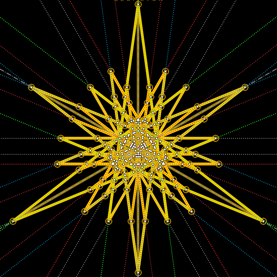
Book II: Regular Polygons & Planar Tilings

Instruction in Measurement (Nuremberg, 1525) — Albrecht Dürer

a: (0, 0) b: (1, 0) d: (\frac{1}{2}, - \frac{\sqrt{3}}{2}) c: (\frac{1}{2}, \frac{\sqrt{3}}{2}) e: (- \frac{1}{2}, - \frac{\sqrt{3}}{2}) f: (\frac{3}{2}, - \frac{\sqrt{3}}{2}) g: (\frac{1}{2}, 1 - \frac{\sqrt{3}}{2}) h: (\frac{1}{4} + \frac{\sqrt{3}}{4} + \frac{\sqrt{2} \sqrt{-2 + 3 \sqrt{3}}}{4}, - \frac{\sqrt{3}}{4} + \frac{\sqrt{2} \sqrt{-2 + 3 \sqrt{3}}}{4} + \frac{3}{4}) i: (- \frac{\sqrt{2} \sqrt{-2 + 3 \sqrt{3}}}{4} - \frac{\sqrt{3}}{4} + \frac{3}{4}, - \frac{\sqrt{3}}{4} + \frac{\sqrt{2} \sqrt{-2 + 3 \sqrt{3}}}{4} + \frac{3}{4}) k: (\frac{- \left(- \frac{\sqrt{2} \sqrt{-2 + 3 \sqrt{3}}}{4} - \frac{\sqrt{3}}{4} + \frac{3}{4}\right)^{2} + \left(- \frac{3}{4} + \frac{\sqrt{3}}{4} + \frac{\sqrt{2} \sqrt{-2 + 3 \sqrt{3}}}{4}\right)^{2} + \left(- \frac{\sqrt{2} \sqrt{-2 + 3 \sqrt{3}}}{2} - \frac{\sqrt{3}}{2} + \frac{1}{2}\right)^{2}}{2 \left(- \frac{\sqrt{2} \sqrt{-2 + 3 \sqrt{3}}}{2} - \frac{\sqrt{3}}{2} + \frac{1}{2}\right)} + \frac{1}{4} + \frac{\sqrt{3}}{4} + \frac{\sqrt{2} \sqrt{-2 + 3 \sqrt{3}}}{4}, - \frac{\sqrt{3}}{4} - \frac{\sqrt{- \left(- \left(- \frac{\sqrt{2} \sqrt{-2 + 3 \sqrt{3}}}{4} - \frac{\sqrt{3}}{4} + \frac{3}{4}\right)^{2} + \left(- \frac{3}{4} + \frac{\sqrt{3}}{4} + \frac{\sqrt{2} \sqrt{-2 + 3 \sqrt{3}}}{4}\right)^{2} + \left(- \frac{\sqrt{2} \sqrt{-2 + 3 \sqrt{3}}}{2} - \frac{\sqrt{3}}{2} + \frac{1}{2}\right)^{2}\right)^{2} + 4 \left(\left(- \frac{3}{4} + \frac{\sqrt{3}}{4} + \frac{\sqrt{2} \sqrt{-2 + 3 \sqrt{3}}}{4}\right)^{2} + \left(- \frac{\sqrt{3}}{4} + \frac{\sqrt{2} \sqrt{-2 + 3 \sqrt{3}}}{4} + \frac{3}{4}\right)^{2}\right) \left(- \frac{\sqrt{2} \sqrt{-2 + 3 \sqrt{3}}}{2} - \frac{\sqrt{3}}{2} + \frac{1}{2}\right)^{2}}}{2 \left(- \frac{\sqrt{2} \sqrt{-2 + 3 \sqrt{3}}}{2} - \frac{\sqrt{3}}{2} + \frac{1}{2}\right)} + \frac{\sqrt{2} \sqrt{-2 + 3 \sqrt{3}}}{4} + \frac{3}{4}) phi: (\frac{1}{2} + \frac{\sqrt{5}}{2}, 0) H_phi: (\frac{\sqrt{5}}{4} + \frac{3}{4}, \frac{\sqrt{2} \sqrt{5 - \sqrt{5}}}{8} + \frac{\sqrt{10} \sqrt{5 - \sqrt{5}}}{8}) I_phi: (\frac{1}{4} - \frac{\sqrt{5}}{4}, \frac{\sqrt{2} \sqrt{5 - \sqrt{5}}}{8} + \frac{\sqrt{10} \sqrt{5 - \sqrt{5}}}{8}) K_phi: (\frac{1}{2}, \frac{\sqrt{2 \sqrt{5} + 5}}{2}) a b d c e f g h i k phi Hphi Iphi Kphi Solid Gold: Dürer Rusty Compass (108.37°) | Dashed Blue: Euclid Q(phi) (108°)

Sections

Plane Enclosure, Exterior Corners vs. Interior Angles & Quadrilaterals (Figs. 1–8)

Having shown in the first book how various lines are to be drawn, I now proceed—as promised at the outset—to planes (planos oder ebne felder), and teach how to construct several of their many figures. To understand what a plane figure is: it is a magnitude bounded and set apart by lines that does not yet enclose a solid body (Corpus). Just as lines enclose a plane, so planes enclose solid bodies.

a: (0, 0) b: (1, 0) d: (\frac{1}{2}, - \frac{\sqrt{3}}{2}) c: (\frac{1}{2}, \frac{\sqrt{3}}{2}) e: (- \frac{1}{2}, - \frac{\sqrt{3}}{2}) f: (\frac{3}{2}, - \frac{\sqrt{3}}{2}) g: (\frac{1}{2}, 1 - \frac{\sqrt{3}}{2}) h: (\frac{1}{4} + \frac{\sqrt{3}}{4} + \frac{\sqrt{2} \sqrt{-2 + 3 \sqrt{3}}}{4}, - \frac{\sqrt{3}}{4} + \frac{\sqrt{2} \sqrt{-2 + 3 \sqrt{3}}}{4} + \frac{3}{4}) i: (- \frac{\sqrt{2} \sqrt{-2 + 3 \sqrt{3}}}{4} - \frac{\sqrt{3}}{4} + \frac{3}{4}, - \frac{\sqrt{3}}{4} + \frac{\sqrt{2} \sqrt{-2 + 3 \sqrt{3}}}{4} + \frac{3}{4}) k: (\frac{- \left(- \frac{\sqrt{2} \sqrt{-2 + 3 \sqrt{3}}}{4} - \frac{\sqrt{3}}{4} + \frac{3}{4}\right)^{2} + \left(- \frac{3}{4} + \frac{\sqrt{3}}{4} + \frac{\sqrt{2} \sqrt{-2 + 3 \sqrt{3}}}{4}\right)^{2} + \left(- \frac{\sqrt{2} \sqrt{-2 + 3 \sqrt{3}}}{2} - \frac{\sqrt{3}}{2} + \frac{1}{2}\right)^{2}}{2 \left(- \frac{\sqrt{2} \sqrt{-2 + 3 \sqrt{3}}}{2} - \frac{\sqrt{3}}{2} + \frac{1}{2}\right)} + \frac{1}{4} + \frac{\sqrt{3}}{4} + \frac{\sqrt{2} \sqrt{-2 + 3 \sqrt{3}}}{4}, - \frac{\sqrt{3}}{4} - \frac{\sqrt{- \left(- \left(- \frac{\sqrt{2} \sqrt{-2 + 3 \sqrt{3}}}{4} - \frac{\sqrt{3}}{4} + \frac{3}{4}\right)^{2} + \left(- \frac{3}{4} + \frac{\sqrt{3}}{4} + \frac{\sqrt{2} \sqrt{-2 + 3 \sqrt{3}}}{4}\right)^{2} + \left(- \frac{\sqrt{2} \sqrt{-2 + 3 \sqrt{3}}}{2} - \frac{\sqrt{3}}{2} + \frac{1}{2}\right)^{2}\right)^{2} + 4 \left(\left(- \frac{3}{4} + \frac{\sqrt{3}}{4} + \frac{\sqrt{2} \sqrt{-2 + 3 \sqrt{3}}}{4}\right)^{2} + \left(- \frac{\sqrt{3}}{4} + \frac{\sqrt{2} \sqrt{-2 + 3 \sqrt{3}}}{4} + \frac{3}{4}\right)^{2}\right) \left(- \frac{\sqrt{2} \sqrt{-2 + 3 \sqrt{3}}}{2} - \frac{\sqrt{3}}{2} + \frac{1}{2}\right)^{2}}}{2 \left(- \frac{\sqrt{2} \sqrt{-2 + 3 \sqrt{3}}}{2} - \frac{\sqrt{3}}{2} + \frac{1}{2}\right)} + \frac{\sqrt{2} \sqrt{-2 + 3 \sqrt{3}}}{4} + \frac{3}{4}) phi: (\frac{1}{2} + \frac{\sqrt{5}}{2}, 0) H_phi: (\frac{\sqrt{5}}{4} + \frac{3}{4}, \frac{\sqrt{2} \sqrt{5 - \sqrt{5}}}{8} + \frac{\sqrt{10} \sqrt{5 - \sqrt{5}}}{8}) I_phi: (\frac{1}{4} - \frac{\sqrt{5}}{4}, \frac{\sqrt{2} \sqrt{5 - \sqrt{5}}}{8} + \frac{\sqrt{10} \sqrt{5 - \sqrt{5}}}{8}) K_phi: (\frac{1}{2}, \frac{\sqrt{2 \sqrt{5} + 5}}{2}) a b d c e f g h i k phi Hphi Iphi Kphi Solid Gold: Dürer Rusty Compass (108.37°) | Dashed Blue: Euclid Q(phi) (108°)

Demonstrative vs. Mechanice Regular Polygons & the Rusty Compass (Figs. 9–20)

Throughout his polygon constructions, Dürer enforces a remarkably modern epistemological boundary between demonstrative constructions proved with exact Euclidean rigor and rapid mechanice workshop approximations (von behendigkeyt wegen in der arbeyt):

a: (0, 0) b: (1, 0) c: (-1, 0) d: (\frac{1}{2}, \frac{\sqrt{3}}{2}) e: (\frac{1}{2}, 0) W_0: (0, 1) W_1: (- \frac{\sqrt{39}}{8}, \frac{5}{8}) W_2: (- \frac{5 \sqrt{39}}{32}, - \frac{7}{32}) W_6: (\frac{1035 \sqrt{39}}{8192}, \frac{5033}{8192}) O_q: (\frac{14}{5}, 0) a b c d e W0 W1 W2 W6 Oq Heptagon: s_7 = sqrt(3)/2 R (P_7(3/4) = -1/64) Quadrature: d = (8/10) diag => pi = 25/8 = 3.125

Euclidean Area Transformations & Circle Quadrature (Figs. 28–36)

The closing movement of Book II treats comparison and transformation of plane areas (vergleichung der ebnen):